相关#
import pandas as pd
from plotnine import *
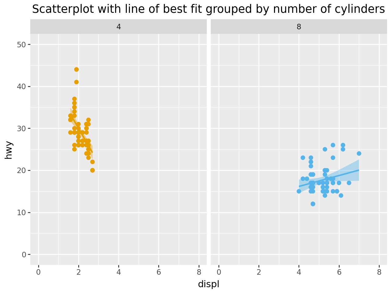
Regression Plot#
mpg = pd.read_csv("data/mpg.csv")
mpg.head()
| manufacturer | model | displ | year | cyl | trans | drv | cty | hwy | fl | class | |
|---|---|---|---|---|---|---|---|---|---|---|---|
| 0 | audi | a4 | 1.8 | 1999 | 4 | auto(l5) | f | 18 | 29 | p | compact |
| 1 | audi | a4 | 1.8 | 1999 | 4 | manual(m5) | f | 21 | 29 | p | compact |
| 2 | audi | a4 | 2.0 | 2008 | 4 | manual(m6) | f | 20 | 31 | p | compact |
| 3 | audi | a4 | 2.0 | 2008 | 4 | auto(av) | f | 21 | 30 | p | compact |
| 4 | audi | a4 | 2.8 | 1999 | 6 | auto(l5) | f | 16 | 26 | p | compact |
mpg_select = mpg.query("cyl in [4, 8]")

(
    ggplot(mpg_select, aes(x="displ", y="hwy", color="cyl", fill="cyl"))
    + geom_point(size=2)
    + geom_smooth(method="lm", size=1)
    + facet_wrap("cyl")
    + lims(x=(0, 8), y=(0, 50))
    + labs(title="Scatterplot with line of best fit grouped by number of cylinders")
    + theme(plot_title=element_text(hjust=0.5), legend_position="none")
    + scale_color_gradient(low="#E69F00", high="#56B4E9")
    + scale_fill_gradient(low="#E69F00", high="#56B4E9")
)
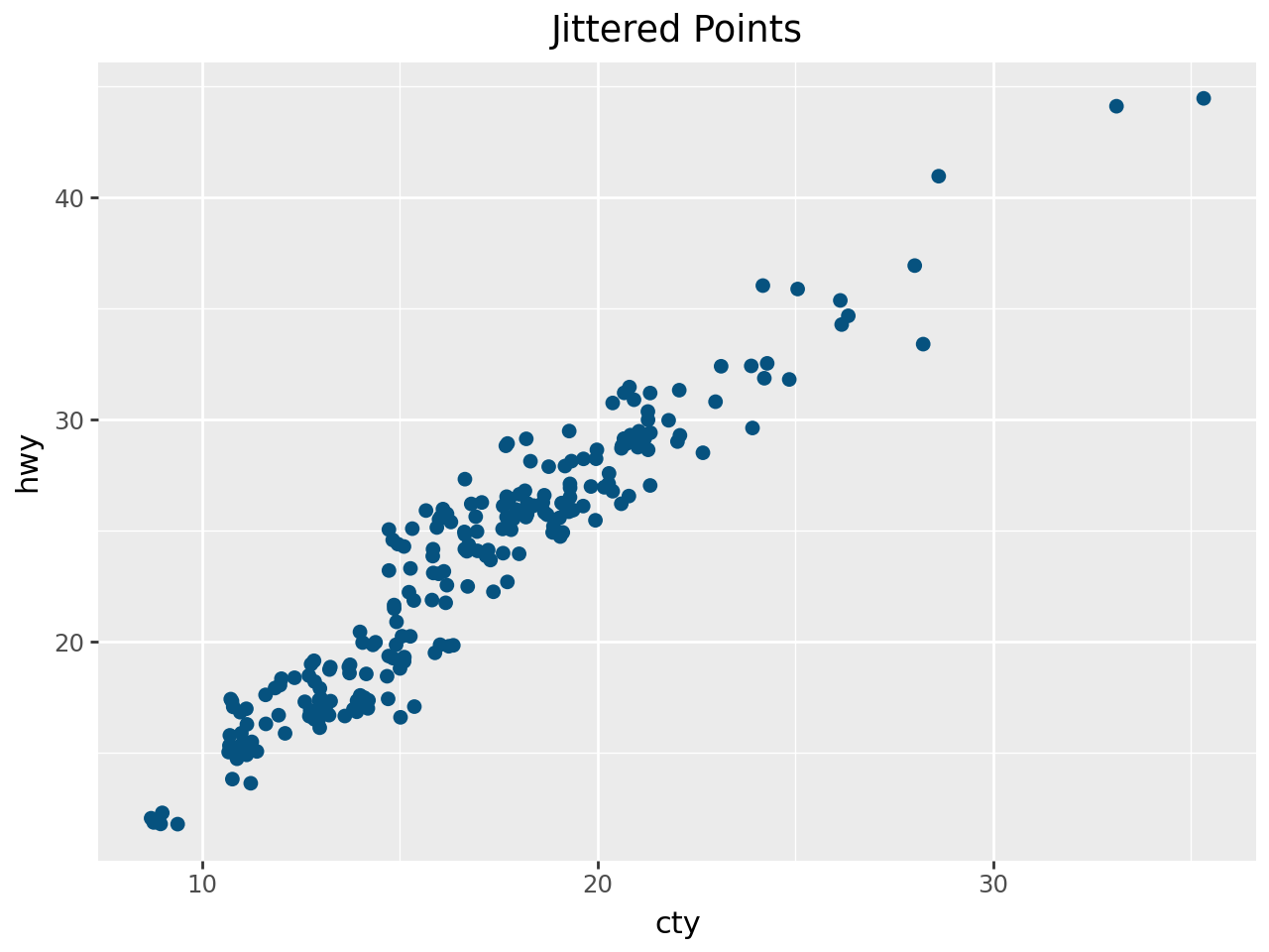
Jittering#
g = ggplot(mpg, aes(x="cty", y="hwy"))

(
    g
    + geom_jitter(height=0.5, size=2, color="#06527f")
    + labs(title="Jittered Points")
    + theme(plot_title=element_text(hjust=0.5))
)
(
g
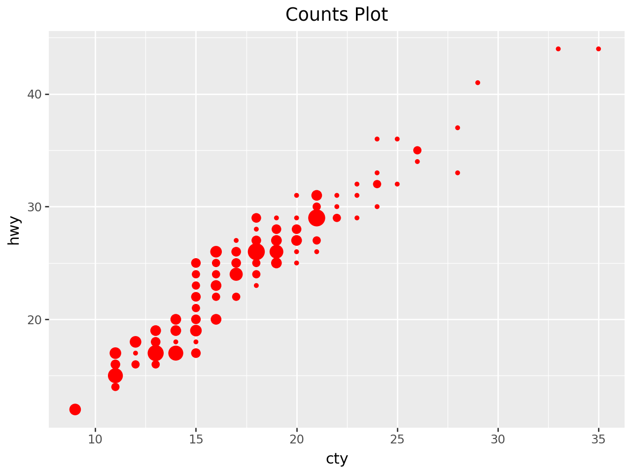
+ geom_count(color="red")
+ labs(title="Counts Plot")
+ theme(plot_title=element_text(hjust=0.5), legend_position="none")
)
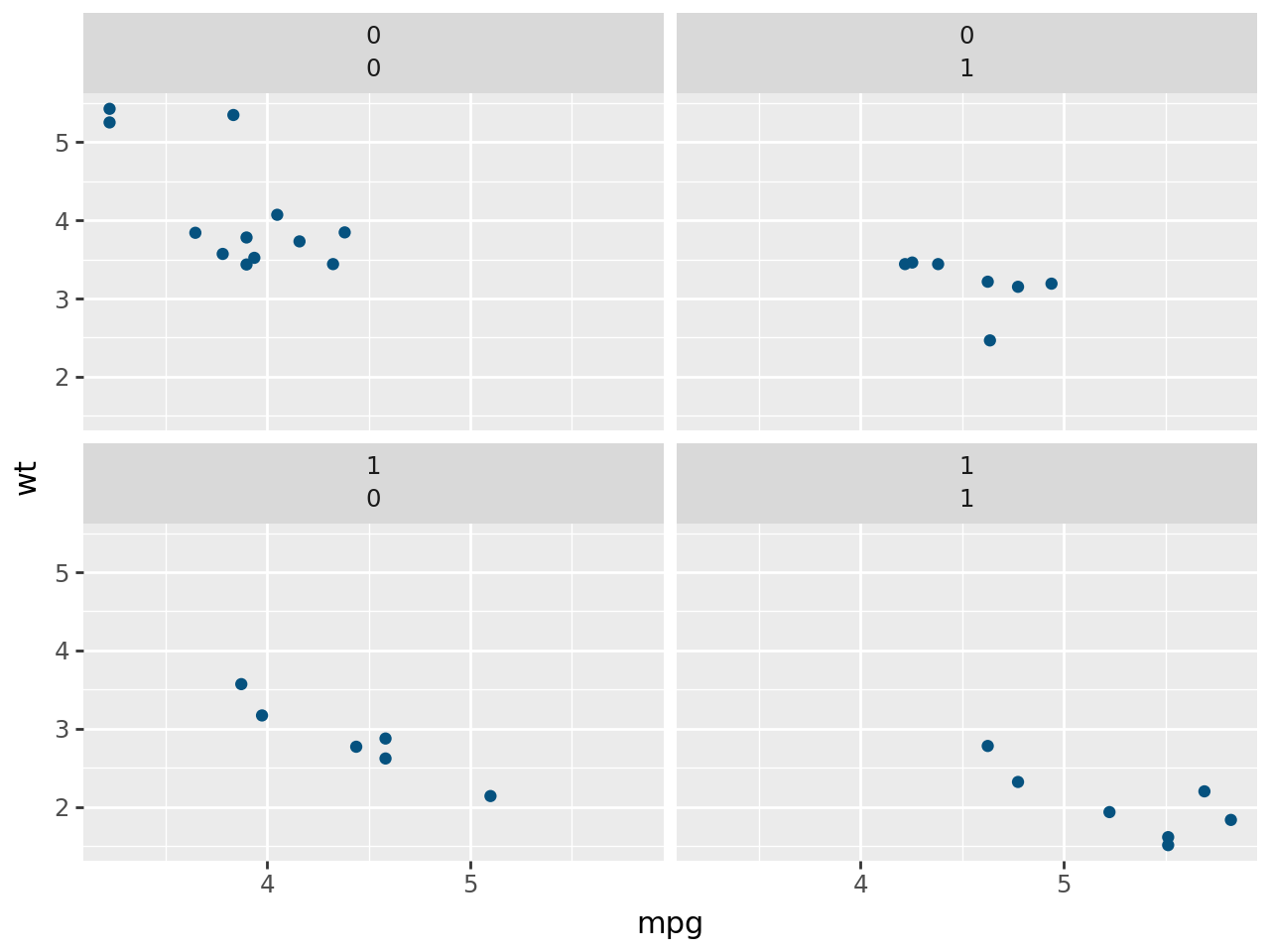
FacetGrid#
mtcars = pd.read_csv("data/mtcars.csv")
mtcars.head()
| mpg | cyl | disp | hp | drat | wt | qsec | vs | am | gear | carb | fast | cars | |
|---|---|---|---|---|---|---|---|---|---|---|---|---|---|
| 0 | 4.582576 | 6 | 160.0 | 110 | 3.90 | 2.620 | 16.46 | 0 | 1 | 4 | 4 | 1 | Mazda RX4 |
| 1 | 4.582576 | 6 | 160.0 | 110 | 3.90 | 2.875 | 17.02 | 0 | 1 | 4 | 4 | 1 | Mazda RX4 Wag |
| 2 | 4.774935 | 4 | 108.0 | 93 | 3.85 | 2.320 | 18.61 | 1 | 1 | 4 | 1 | 1 | Datsun 710 |
| 3 | 4.626013 | 6 | 258.0 | 110 | 3.08 | 3.215 | 19.44 | 1 | 0 | 3 | 1 | 1 | Hornet 4 Drive |
| 4 | 4.324350 | 8 | 360.0 | 175 | 3.15 | 3.440 | 17.02 | 0 | 0 | 3 | 2 | 1 | Hornet Sportabout |
(
    ggplot(mtcars, aes("mpg", "wt"))
    + geom_point(color="#06527f")
    + facet_wrap(["am", "vs"])
)
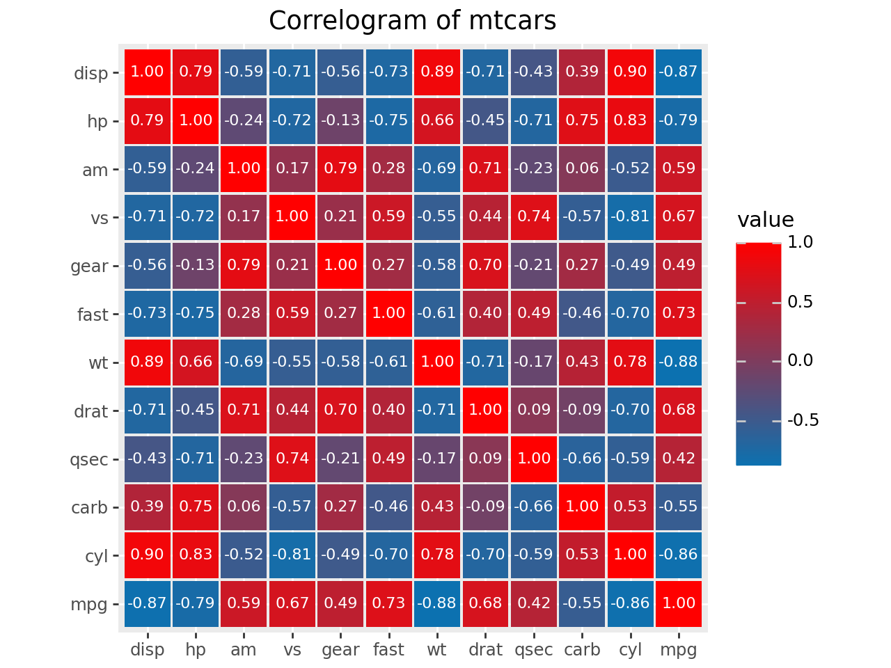
Heatmap#
corr_matrix = mtcars.corr(numeric_only=True)
corr_matrix.head()
| mpg | cyl | disp | hp | drat | wt | qsec | vs | am | gear | carb | fast | |
|---|---|---|---|---|---|---|---|---|---|---|---|---|
| mpg | 1.000000 | -0.858539 | -0.867536 | -0.787309 | 0.680312 | -0.883453 | 0.420317 | 0.669260 | 0.593153 | 0.487226 | -0.553703 | 0.730748 |
| cyl | -0.858539 | 1.000000 | 0.902033 | 0.832447 | -0.699938 | 0.782496 | -0.591242 | -0.810812 | -0.522607 | -0.492687 | 0.526988 | -0.695182 |
| disp | -0.867536 | 0.902033 | 1.000000 | 0.790949 | -0.710214 | 0.887980 | -0.433698 | -0.710416 | -0.591227 | -0.555569 | 0.394977 | -0.732073 |
| hp | -0.787309 | 0.832447 | 0.790949 | 1.000000 | -0.448759 | 0.658748 | -0.708223 | -0.723097 | -0.243204 | -0.125704 | 0.749812 | -0.751422 |
| drat | 0.680312 | -0.699938 | -0.710214 | -0.448759 | 1.000000 | -0.712441 | 0.091205 | 0.440278 | 0.712711 | 0.699610 | -0.090790 | 0.400430 |
corr_matrix2 = (
    corr_matrix.reset_index()
    .melt(id_vars="index")
    .sort_values("value", ascending=False)
)
corr_matrix2.head()
| index | variable | value | |
|---|---|---|---|
| 0 | mpg | mpg | 1.0 |
| 13 | cyl | cyl | 1.0 |
| 130 | carb | carb | 1.0 |
| 78 | qsec | qsec | 1.0 |
| 52 | drat | drat | 1.0 |
sort_seq = corr_matrix2.variable.unique()
(
    ggplot(corr_matrix2, aes("index", "variable", fill="value"))
    + geom_tile(aes(width=0.95, height=0.95))
    + scale_fill_gradient(low="#0c71b0", high="#ff0000")
    + geom_text(aes(label="value"), size=8, format_string="{:.2f}", color="white")
    + labs(title="Correlogram of mtcars", x="", y="")
    + scale_x_discrete(limits=sort_seq[::-1])
    + scale_y_discrete(limits=sort_seq)
    + coord_fixed()
)
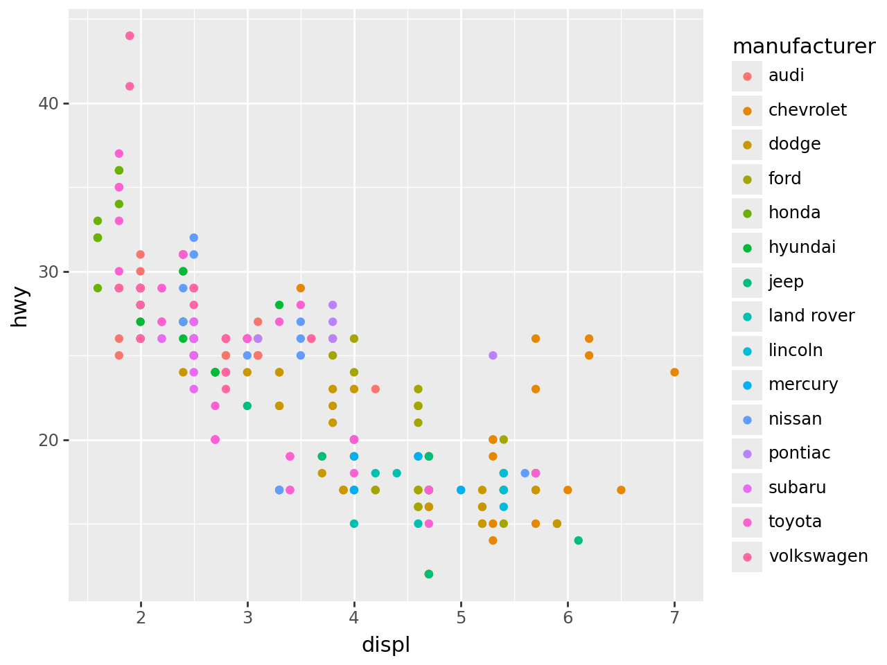
Marginal Plot#
g1 = ggplot(mpg) + geom_point(aes("displ", "hwy", color="manufacturer"))
g2 = ggplot(mpg) + geom_boxplot(aes("displ", "hwy"))
g3 = ggplot(mpg) + geom_boxplot(aes("hwy", "displ")) + coord_flip()
g1